Bryn Battersby
Treasury Working Paper
2006 — 03
April 2006
The author is grateful to Jyoti Rahman, Graeme Davis, David Gruen, LewisEvans, Ben Dolman, Robert Ewing, Janine Murphy and Gene Tunny for helpful comments in preparing this paper. The views expressed are those of the author and not necessarily those of the Treasury or the Government.
Abstract
Over the past 50 years, Australia has maintained a labour productivity level of around 80 percent of that of the United States. To explain this gap, there is growing interest in the hindrances that might be imposed by Australia’s geographic isolation. If the level of labour productivity is constrained by geographic isolation, then the scope to close the productivity gap with the United States is less than previously thought.
This paper provides an initial investigation of the link between distance and labour productivity levels. Parameters of a simple labour productivity equation are estimated for the states of the United States of America and Australia. This equation includes an indicator that captures, for each state, the economic size of the state, the state’s proximity to other states and the economic size of those other states. The regressions find that this indicator is a significant determinant of state productivity levels and that Australia’s isolation from world economic activity accounts for around 45 per cent of the gap in labour productivity between Australia and the United States.
JEL Classification Numbers: O47
Keywords: Productivity, geographic isolation, distance, agglomeration
Contents
4. Estimating proximity and the labour productivity equation
Does distance matter?
The effect of geographic isolation on productivity levels
Bryn Battersby
1. Introduction
Australia’s productivity level has hovered around 80 per cent of the United States’ productivity level for much of the last 50 years. Australia’s economic performance can be and often is traced by its position relative to this 80 per cent level. For instance, in the slowdown of the 1970s and the 1980s, Australia’s productivity level fell to under 80 per cent of the US productivity level. Then, through the process of reform, Australian productivity climbed back to around 80 per cent of the US level.
However, the pervasiveness and size of this gap suggests that there may be more to it than just differences in economic policy.
One possible explanation for some of the productivity gap might be found in the natural circumstances of the two countries. The United States is a large country (around 15 times larger in population and 18 times larger in output than Australia) and can consequently take advantage of the better potential for economies of scale and scope. Indeed, the 2003-04 Australian Budget Papers highlighted Australia’s internal and external geographic circumstance and noted that ‘fully achieving economies of scale and scope in many industries requires large markets, either domestically or internationally through trade’ (Budget Statement 4, p 4-19). It is readily apparent that these advantages do not reside with Australia.
Gravity trade models have provided a good example of the effect of Australia’s distance on one economic measure — trade. These equations have explained how Australia’s distance to the world’s ‘economic mass’ has an impact on Australia’s expected level of trade. In earlier work along these lines, Battersby and Ewing (2005) noted:
‘Accounting for the factors [of distance and size] in the gravity trade equation suggests that Australia’s comparative trade performance is actually quite strong. These factors, which are ordinarily outside the control of policy, plainly have a role in determining many economic outcomes in a country. In Australia’s case, geographic remoteness increases the costs of trading, which in turn lowers the extent of international trade and provides varying degrees of natural protection for Australian industries.’ (p 17)
It was suggested that this reinforces the importance of accounting for Australia’s ‘tyranny of distance’ (Blainey 2003) both when comparing Australia internationally and when defining appropriate policy solutions for Australia. However, until recently, little evidence had been provided to suggest that any other area of Australia’s economic performance is adversely affected by this geographic isolation.
Recent work on the economic performance of New Zealand (another geographically isolated country) by the International Monetary Fund has shed some light on the effect of geographic isolation on economic performance. The IMF (2004) found ‘strong support for the view that geographic isolation has significantly hampered growth in New Zealand.’ Their regressions also suggest that Australia’s economic growth is hampered by this isolation.
The work outlined in this paper takes a slightly different approach from that of the IMF. Analysis is undertaken at the state level to include the effect of a country’s internal geographic proximity on the level of labour productivity. Analysis at the state level reduces (but does not eliminate) the policy and cultural differences that are usually not captured in an international cross-country analysis. The level of productivity rather than the growth rate of productivity is analysed because it is expected that distance acts like a natural protection for the Australian economy. This imposes a condition on convergence with the productivity frontier but does not mean that the rate of growth is any lower than the frontier’s in the long run.
To test the proposition that distance matters, a proximity variable is calculated that includes the state’s own output and all other economic output in the world weighted by its distance from the state. The indicator that is developed is a combined measure of weighted own-state output, weighted other-state output and weighted other-country output, where the weights depend on the distance to the output.
The results of a cross-section regression of state productivity levels on the factors of production and the proximity variable suggest that around 40 per cent of the productivity gap between the United States and Australia might be explained by Australia’s geographic isolation.
Background literature
This work has some connection with the economics of agglomeration, which was first explored by Marshall (1920). Marshall suggested that the concentration of economic activity enhanced productivity through the pooling of labour, knowledge and technological spillovers, and input sharing. More recently, research has estimated the effect of density on st
ate and city levels of productivity. For instance, Ciccone and Hall (1996) found that the intensity of labour, human and physical capital of a state had a positive and significant effect on labour productivity. Rosenthal and Strange (2003) have also explored the effect of density on different industries in US cities. They found that spatial concentration produces a number of agglomeration externalities and that these differ across industries. Other similar types of empirical research on the role of regional concentration in output and productivity can be found in Ciccone(2002) and Rice and Venables (2004).
However, the research in this area has predominantly focused on examining the positive externalities of concentration in small areas. The interest in this paper, though, is on the effect of Australia’s internal distance and distance from world output on the gap between Australian and US labour productivity levels. The indicator of concentration that is developed in this paper is therefore not an indicator of concentration within a city, or even concentration within a state, but rather how close a state is to the rest of the world’s output. Moreover, while other research has tended to suggest an attenuation of the agglomeration effects beyond small distances, the research contained here is based on the premise that over much greater distances, geographical isolation reduces the labour productivity potential of an economy. Geographic isolation may do this by reducing the relative mobility of labour, reducing the absorptive capacity of an economy, and increasing the price (and reducing the competitiveness) of imports.
This paper has six sections. The second section outlines a simple Cobb-Douglas specification for an empirical analysis of state productivity levels. This is then followed in the third section by a comprehensive analysis of the data. The fourth section presents the set of results from the estimation of the specification of state labour productivity. The fifth section discusses these results, which suggest that labour productivity is negatively affected by an economy’s isolation. Finally, the sixth section concludes the paper and offers some directions for further research.
2. Model Specification
A simple specification based on the Cobb-Douglas production function is used to estimate the level of labour productivity by state. This specification allows a comparison with other similar regression results and is relatively easy to estimate. The basic specification of the model without regional effects is presented in equation (1).
![]() (1)
(1)
In equation (1), Yi represents the gross state income of state i, K is an indicator of the capital stock, L is an indicator of the stock of labour, H is an indicator of the stock of human capital and ![]() are coefficients on these variables. Dividing this equation through by the labour stock and taking logs, equation (2) presents a simple labour productivity model that considers the two capital to labour ratios.
are coefficients on these variables. Dividing this equation through by the labour stock and taking logs, equation (2) presents a simple labour productivity model that considers the two capital to labour ratios.
![]() (2)
(2)
Additional variables, such as indicators of market concentration and country specific dummies, can then be added to this specification. Equation (3) presents the final specification of the equation, with betas identifying the coefficients for estimation, ![]() representing the indicator of the proximity of state i to world economic output, and Aus representing a dummy variable that indicates whether the state is Australian or not.
representing the indicator of the proximity of state i to world economic output, and Aus representing a dummy variable that indicates whether the state is Australian or not.
![]() (3)
(3)
Rather than being an analysis of productivity through time, this analysis is a cross-section analysis over the states of the United States of America and Australia. While this does not challenge the integrity of the basic functional form (productivity levels are still expected to differ because of factor intensities), the goodness of fit is expected to be lower than time-series estimation as there are no lag dependencies.
3. Data
There are numerous challenges in the construction of the dataset for this project. For example, constraints on data availability mean that the income, capital and labour indicators for the United States and Australia are constructed from data that excludes the public and agricultural sectors. In addition, capital stock data are not readily available for the individual states of Australia or the United States and had to be calculated from industry averages.
3.1 Labour
The most useful labour data for calculating productivity levels and capital to labour ratios are the number of hours worked in an economy. Unlike the more accessible total-workers data, hours-worked data capture differences in the proclivity for work between different economies.1
However, there is a number of problems in deriving total hours worked data for each state of Australia and the United States.
Firstly, while state-level total hours-worked data do exist for Australia, there are no state-level total hours-worked data for the United States. Nevertheless, total-workers data are available at a state level for the United States. These total-workers data are also disaggregated to the level of the ‘super-sector’. Finally, applying US national sectoral hours-worked per worker data to these state sectoral total workers data provides the basis for calculating the total hours worked in each state.
However, a second problem arises with these data. Due to a lack of farm sector data for the US and hours-worked data for the Australian public sector, these two sectors are eliminated from the analysis in both countries. This ensures consistent treatment of the available data across the two countries. The significance of removing these two sectors is demonstrated in Charts 1 and 2.
Finally, some scaling of the sectoral hours-worked data is also necessary to maintain consistency with other estimates of average hours worked in the economy (such as those from the Groningen Growth and Development Centre).2
Chart 1: Employment by Super-Sector
United States of America, 2001
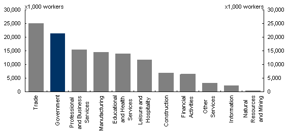
Source: Bureau of Labour Statistics Current Employment Statistics Survey, 2004
Chart 2: Employment by ANZSIC sector
Australia, 2001
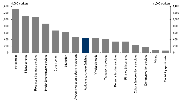
Source: Labour Force Statistics (ABS cat. no. 6203.)
3.2 Capital stock and the capital to labour ratios
To calculate state capital stocks, industry capital to labour (K/L) ratios are applied to state sectoral labour estimates. While this implicitly assumes constant K/L ratios for industries across states, it allows an estimate of the state capital stocks to be developed and used in the labour productivity regression.
Capital stock data for each state of the United States are constructed from two-digit standard industry classification (SIC) detail as direct aggregates in billions of 1996 dollars. National capital to labour ratios a
re calculated for each of the labour super-sectors used by the US Bureau of Labor Statistics. This requires matching the older capital stock SIC codes with the newer North American Industry Classification System (NAICS) codes. The overlap of some of the codes may reduce the integrity of some of the capital to labour ratios.
After converting the capital stock by industry to capital stock by super-sector, a capital to labour ratio is calculated for each of the eleven sectors (Construction; Educational and Health Services; Financial Activities; Information Leisure and Hospitality; Manufacturing; Natural Resources and Mining; Other Services; Professional and Business Services; and Trade).
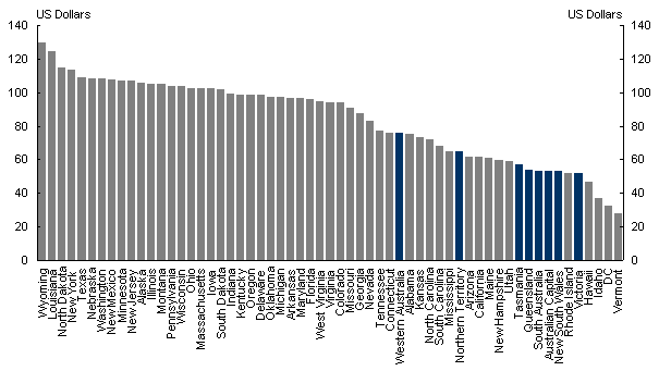
The capital stock for each state is then calculated by multiplying the national capital to labour ratio for each sector by the employment for each sector in the state. The US state capital to labour ratios are presented in Chart 3. As expected, states with high mining intensities and higher levels of financial activity tend to have higher capital to labour ratios.
State capital stocks for Australia are calculated by the same method used for the US state capital stocks. The 2001 Australian national capital stocks in current dollars are obtained from the Australian National Accounts. For consistency with the US state data, this is adjusted to 2001 purchasing power parity (PPP) USdollars using OECD (2004) calculated PPPs. These state capital stock data are presented alongside the US data in Chart 3.
The Australian data consist of 16 sectors: Retail trade; Manufacturing; Property and business services; Health and community services; Construction; Education; Accommodation, cafes and restaurant; Agriculture, forestry and fishing; Wholesale trade; Transport and storage; Government administration and defence; Personal and other services; Finance and insurance; Cultural and recreational services; Communication services; Mining; and Electricity, gas and water. The agriculture, forestry and fishing and government administration and defence sectors are excluded from the analysis to retain consistency with the US data.
Chart 3: Capital per hour worked by state:
United States and Australia, 2001
Source: Bureau of Labor Statistics, www.bls.gov, Australian National Accounts (ABS cat. no. 5204) and Australia Labour Force Statistics (ABS cat. 6203).
As is the case for US states, Australian states that are particularly mining intensive have a higher reported capital to labour ratio. However, the capital to labour ratios of the Australian states are generally low. Indeed, the Australian states that are particularly mining intensive (WA and NT) have capital to labour ratios comparable with the US average. Given the small workforce of these states and the size of their mining industries, it might have been expected that these capital to labour ratios would be much higher.
The lower than expected Australian capital to labour ratios, however, might be a consequence of assumptions and data problems. For instance, the assumption of constant industry capital to labour ratios across states and the possible measurement discrepancies across countries might bias the capital to labour ratios for any of the states. These concerns signal an important caveat and limitation on the interpretation of the results in this analysis. The acquisition or construction of better capital stock data would be a useful direction for further work.
3.3 Income
Gross state product figures for each of the US states are acquired from the Bureau of Economic Analysis. The US gross state products used in this analysis are for the year 2001 and exclude the agricultural and government sectors.
Australian state income levels are calculated as the state total factor income less the agricultural and public sectors. These are scaled to distribute the residual between Australian GDP and the total of all state incomes proportionally to each state. This residual is almost solely attributable to the Australian National Accounts item ‘taxes less subsidies’.
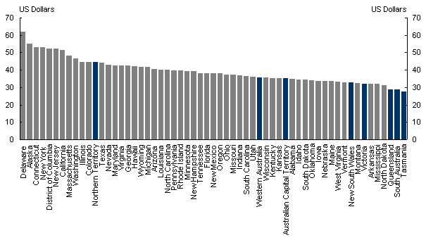
These data are then adjusted to 2001 PPP US dollars to be consistent with the US data. Chart 4 presents the resultant output per hour worked for Australian and US states.
A comparison of Australian and US state productivity using these measures suggests that the Australian productivity level is around 75 per cent of the United States. This measure is therefore 5 percentage points less than the regularly cited 80 per cent relative productivity level.3 However, given the aforementioned difficulties in calculating comparative measures of productivity, and given the nature of this analysis, this difference is tolerable.
Chart 4: 2001 Output per hour worked by state
United States and Australia
Source: Bureau of Economic Analysis, www.bea.gov and ABS State Accounts (ABS cat. no. 5220)
3.4 Human capital
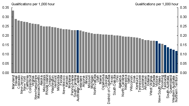
Good measures of human capital are difficult to generate because human capital is a complex concept. It can include the stock of research, the range of skills, or even the ability to distribute ideas in an economy. Here, we simply use the number of people holding a bachelor’s degree or better per 1,000 hours worked as an indicator of the stock of human capital.4 These data, which are available at a state level in both the United States and Australia, are presented in Chart 5.
Chart 5: Human capital: Number of bachelor’s degrees or better
per 1,000 hours worked, 2001
Source: US Census Bureau, www.census.gov and Education and Work, (ABS cat. no. 6227).
3.5 Summary of the data
Appendix A provides a summary of the data used in the analysis.
4. Estimating proximity and the labour productivity equation
4.1 An indicator of proximity
The proximity variable is the key variable of interest. This variable is intended to capture the proximity of the state to world output. Closeness to output is hypothesised to present scale opportunities and spillovers for firms and this, in turn, enables a higher level of productivity, other things held constant.
An indicator of proximity could be derived by arbitrarily defining a boundary and aggregating all output that falls within that boundary. However, both the exclusion of all output beyond that boundary and the arbitrariness of the boundary encourage a search for a better measure of proximity.
The alternative measure we use aggregates ‘decayed’ outputs of the economies in the dataset with the decay depending on distance from the state of interest. Formally, the proximity indicator for state i is defined in equation (4):
![]() (4)
(4)
The sample consists of j=1,…,n ‘economies’, which are either Australian or US states or other count
ries. ![]() is the output of economy j and
is the output of economy j and ![]() is the distance to economy j to the power -
is the distance to economy j to the power -![]() .
.
The dataset used to create this variable includes each of the US and Australian states, as well as all other countries in the world for which data are available. The most recently available data are for the year 1998. Distances, measured in kilometres, are calculated between capital cities.
Estimation of equation (3) could be undertaken in a straightforward way using ordinary least squares. However, this would require assuming a value for ![]() in equation (4) as well as for the distance of the state from its own output, dii.
in equation (4) as well as for the distance of the state from its own output, dii.
In this analysis, two estimation steps are used. First, both ![]() and the distance to own GDP, dii, are estimated alongside the coefficients in the productivity equation. Then, a proximity indicator is constructed for each state, and used in ordinary least squares estimations of the parameters
and the distance to own GDP, dii, are estimated alongside the coefficients in the productivity equation. Then, a proximity indicator is constructed for each state, and used in ordinary least squares estimations of the parameters![]() . This second step was taken to simplify both the testing and the analysis of the results.
. This second step was taken to simplify both the testing and the analysis of the results.
In the first step, ![]() ,
, ![]() and
and ![]() are parameters to be estimated by maximum likelihood using the following specification with a standard normal distribution of the error (Appendix B presents additional detail).
are parameters to be estimated by maximum likelihood using the following specification with a standard normal distribution of the error (Appendix B presents additional detail).
 (5)
(5)
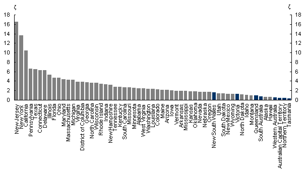
The estimated proximity indicators for each state are presented in Chart 6. These indicators seem to accord with a priori expectations. That is, states such as New York, New Jersey and California are especially proximate to economic output, as are their surrounding states. The Australian states, however, are further away from world economic output. Notably, the large output of New South Wales makes it closer to world output than a few of the most remote states of the United States.
Chart 6: Proximity indicator with optimal alpha and distance to own output values
4.2 Model results
Table 1 presents the set of estimates from ordinary least squares regressions of variations of equation (1). Some of these regressions use the proximity indicators presented in Chart 6.
Equation A presents estimates of the coefficients in the simple model of output. Coefficients on both the capital to labour ratio and the human capital to labour ratio are positive and significant, as expected.
Equation B includes the dummy variable identifying Australian states. Both capital to labour ratios have reduced significance, but the dummy variable is not significant. While the standard error of the coefficient on the dummy variable urges caution in the coefficient’s interpretation, the negative sign suggests that there are reasons other than differences in capital to labour ratios that explain Australia’s productivity gap with the US.
|
Variable |
A |
B |
C |
D |
|
Constant |
3.861 |
3.861 |
3.742 |
3.741 |
|
Log(K/L) |
0.087 |
0.081 |
0.041 |
0.031 |
|
Log(H/L) |
0.374 |
0.357 |
0.222 |
0.193 |
|
Proximity |
0.027 |
0.027 |
||
|
Australia |
-0.018 |
-0.029 |
||
|
R-squared |
0.265 |
0.266 |
0.426 |
0.428 |
|
RESET |
2.000 |
3.441 |
2.810 |
3.427 |
|
Heteroskedasticity |
0.932 |
0.797 |
0.855 |
0.760 |
Numbers in brackets are t-statistics. *** indicates significance at the 1 per cent level, ** indicates significance at the 5 per cent level, * indicates significance at the 10 per cent level. RESET and Heteroskedasticity (White’s test) are F-statistics. None of these F-statistics is significant at the 10 per cent level. The proximity indicator variable was divided by 1000 prior to estimation.
Table 2: Correlation coefficients of the variables
|
Proximity |
Human Capital |
|
|
Physical Capital |
0.713 |
0.920 |
|
Human Capital |
0.723 |
Equation C presents the first of two sets of results that include the proximity indicator. The coefficient on the proximity indicator has a positive sign, which implies that the greater the level of output near the state, the greater the level of labour productivity. Also apparent in this regression is the reduction in significance of the capital to labour ratio coefficients. The reduction in explanatory power of these variables is offset by the more significant coefficient on the proximity indicator and may be a result of multicollinearity with the proximity indicator (see below).
Finally, equation D, suggests that the Australian-state dummy variable adds nothing of significance to the regression.
Each of the RESET tests shows no signs of misspecification. F-statistics from White’s test also suggest that the regressions do not suffer from heteroskedasticity. Correlations between the variables, presented in Table 2, suggest that there may be multicollinearity, which adversely affects the standard errors of the variables. While multicollinearity is generally expected in the estimation of a Cobb-Douglas equation, the correlations between the capital indicators and the proximity indicators may deserve further investigation. This is because distance may also increase the transaction costs associated with factor accumulation.
5. Discussion
Several simple equations of state productivity levels have been estimated in order to assess the extent to which proximity to economic mass affects productivity. The coefficient on the variable that captured this proximity (the proximity indicator) was positive and significant. The effect of the proximity indicator in the regressions is evidenced by shifting it by one standard deviation from its mean, which results in a 6 per cent shift in the expected level of labour productivity.
Using the parameters and variables presented in this paper, it is possible to calculate the proportion of the productivity gap between Australia and the United States explained by Australia’s geographic isolation. An average proximity indicator for Australia (![]() ) can be calculated as:
) can be calculated as:
 (6)
(6)
This calculation weights proximity by the total number of hours worked in a state. Average proximity can also be similarly calculated for the United States (![]() ).
).
It is then possible to calculate the labour productivity difference accounted for by the difference in this proximity indicator as:
 (7)
(7)
This simplifies to equation (8), where y represents labour productivity:
![]() (8)
(8)
Using equation (8) and the results and data outlined earlier, the ratio of Australian labour productivity to US labour productivity that arises in the model purely from differences in the proximity indicator is 0.89. The actual ratio of Australian labour productivity to US productivity in the dataset is 0.75, which suggests that differences in proximity account for just under 45 per cent of the difference in labour productivity levels between the United States and Australia.
Of course, this calculation should be used with caution. Appendix B presents some analysis of the sensitivity of this estimate to changes in the values of ![]() and
and ![]() , but further checks of the estimate’s robustness would be useful. The results do suggest, though, that distance may be accounting for a notable part of the labour productivity gap between Australia and the United States. Importantly, these results also suggest that there are other reasons for Australia’s productivity gap with the United States beyond simply the scale and spillover effects that benefit the US economy.
, but further checks of the estimate’s robustness would be useful. The results do suggest, though, that distance may be accounting for a notable part of the labour productivity gap between Australia and the United States. Importantly, these results also suggest that there are other reasons for Australia’s productivity gap with the United States beyond simply the scale and spillover effects that benefit the US economy.
6. Conclusion
This paper began by suggesting that the productivity gap between Australia and the United States may not be as responsive to policy as has been previously thought. Indeed, the relative stability of the gap over time suggests that it may not be possible to completely close it. This paper has investigated the possibility that Australia’s internal and external ‘tyranny of distance’ is an important reason for at least some of the gap.
In regressions of labour productivity on an indicator of proximity (which captures a state’s closeness to world economic output) along with physical and human capital, the coefficient on proximity was positive and significant. This coefficient suggests that the difference in the average proximity indicators for Australia and the United States accounts for around 45 per cent of the labour productivity gap. This further suggests that even over considerable distances (greater than those identified in standard agglomeration economics), there may be significant external effects from being located near centres of output.
However, there remain a number of critical mysteries. For example, differences in the physical and human capital to labour ratios explain a large portion of the difference in labour productivity, but it is not immediately clear why these factor intensity differences exist. One clue might be in the correlations between the proximity indicator and the factor intensities, though further work will be necessary to draw out that story.
This paper represents an initial investigation of the effect of distance from world output on state productivity levels. There remains a range of possible future directions for this type of work, including:
- the construction of better capital stock data;
- the inclusion of more spatially disaggregated data that allows a more complete indication of internal proximity;
- a comparison of the industry structure of states and identification of differences in labour productivity attributable to those different structures;
- further diagnostic testing, including tests for spatial autocorrelation and endogeneity; and
- the investigation of alternative methods for constructing indicators of proximity.
Notwithstanding the possibility of significant methodological improvements in future, this work has provided initial evidence of a significant and economically important link between the proximity of a state to output and its level of labour productivity. The results imply that productivity levels in Australian states are disadvantaged because of their distance both from global centres of output and from each other.
7. References
Australian Government 2003, ‘Sustaining Growth in Australia’s Living Standards’ Budget Paper No. 1, Budget Strategy and Outlook 2003-04, Statement4.
Battersby, B D and Ewing R J, 2005, ‘International Trade Performance: The Gravity of Australia’s Remoteness’ Treasury Working Paper No. 2005-03, Australian Treasury, Canberra.
Blainey, G 1983, The tyranny of distance: How distance shaped Australia's history, Pan-Macmillan.
Ciccone, A 2002, ‘Agglomeration effects in Europe’, European Economic Review, 46(2), pp 213-228.
Ci
ccone, A and R Hall 1996, ‘Productivity and the Density of Economic Activity’, American Economic Review, 86 (1), pp 54-70.
IMF 2004, ‘Sources of Economic Growth in New Zealand: A Comparative Analysis’, IMF Country Report No. 04/127, International Monetary Fund: Washington.
Marshall, A 1920, Principles of Economics, 8th edition, Macmillan: London.
OECD 2004, Purchasing Power Parities and Real Expenditures: 2002 Benchmark Year: Paris.
Rice, P and Venables A J 2004, ‘Spatial Determinants of Productivity: Analysis for the Regions of Great Britain’, CEP Discussion Paper No. 642, London School of Economics.
Rosenthal, S S and Strange W C 2003, ‘Geography, industrial organization and agglomeration’, Review of Economics and Statistics, 85, pp 377-393.
8. Appendix A
Table A1: Summary of data
|
State |
Y/L |
K/L |
H/L*1000 |
Proximity. Ind. |
|
NSW |
32.73 |
53.12 |
0.16 |
1.57 |
|
VIC |
32.06 |
51.65 |
0.17 |
1.23 |
|
QLD |
28.87 |
54.09 |
0.13 |
0.94 |
|
SA |
28.72 |
53.35 |
0.14 |
0.73 |
|
WA |
35.57 |
76.04 |
0.12 |
0.53 |
|
TAS |
27.70 |
57.26 |
0.15 |
0.33 |
|
NT |
44.51 |
64.57 |
0.12 |
0.41 |
|
ACT |
35.21 |
53.13 |
0.23 |
0.44 |
|
Alabama |
34.95 |
74.92 |
0.20 |
2.45 |
|
Alaska |
55.07 |
105.75 |
0.25 |
0.64 |
|
Arizona |
40.35 |
61.68 |
0.22 |
2.10 |
|
Arkansas |
31.84 |
96.80 |
0.18 |
1.93 |
|
California |
51.29 |
61.59 |
0.27 |
10.54 |
|
Colorado |
44.52 |
93.83 |
0.28 |
2.19 |
|
Connecticut |
53.20 |
76.04 |
0.27 |
6.32 |
|
Delaware |
62.01 |
98.29 |
0.23 |
6.28 |
|
District of Columbia |
52.13 |
32.34 |
0.20 |
3.83 |
|
Florida |
38.14 |
95.94 |
0.24 |
4.71 |
|
Georgia |
42.29 |
87.57 |
0.20 |
3.72 |
|
Hawaii |
42.12 |
46.87 |
0.29 |
0.60 |
|
Idaho |
34.40 |
37.24 |
0.19 |
1.05 |
|
Illinois |
44.56 |
105.10 |
0.22 |
5.34 |
|
Indiana |
36.91 |
99.43 |
0.18 |
3.31 |
|
Iowa |
33.78 |
102.23 |
0.19 |
2.06 |
|
Kansas |
35.36 |
73.06 |
0.23 |
1.84 |
|
Kentucky |
35.40 |
98.66 |
0.19 |
2.76 |
|
Louisiana |
40.11 |
124.52 |
0.18 |
2.33 |
|
Maine |
33.39 |
60.72 |
0.21 |
2.17 |
|
Maryland |
42.54 |
96.78 |
0.33 |
4.33 |
|
Massachusetts |
48.15 |
102.52 |
0.26 |
4.29 |
|
Michigan |
41.64 |
96.95 |
0.21 |
4.24 |
|
Minnesota |
39.43 |
107.06 |
0.24 |
2.56 |
|
Mississippi |
31.81 |
64.92 |
0.25 |
1.90 |
|
Missouri |
37.22 |
90.57 |
0.22 |
2.62 |
|
Montana |
32.20 |
104.93 |
0.23 |
0.97 |
|
Nebraska |
33.65 |
108.45 |
0.19 |
1.72 |
|
Nevada |
42.89 |
82.84 |
0.17 |
1.76 |
|
New Hampshire |
39.21 |
59.88 |
0.26 |
3.21 |
|
New Jersey |
52.02 |
106.67 |
0.28 |
16.57 |
|
New Mexico |
38.03 |
107.90 |
0.23 |
1.31 |
|
New York |
53.18 |
113.40 |
0.27 |
13.68 |
|
North Carolina |
40.02 |
71.64 |
0.20 |
3.69 |
|
North Dakota |
31.17 |
115.00 |
0.21 |
1.15 |
Table A1: Summary of data (continued)
|
State |
Y/L |
K/L |
H/L*1000 |
Proximity. Ind. |
|
Ohio |
37.26 |
102.60 |
0.20 |
4.66 |
|
Oklahoma |
34.17 |
97.41 |
0.21 |
1.83 |
|
Oregon |
37.91 |
98.61 |
0.25 |
1.70 |
|
Pennsylvania |
39.86 |
103.90 |
0.23 |
6.62 |
|
Rhode Island |
39.65 |
52.05 |
0.25 |
3.38 |
|
South Carolina |
36.43 |
68.10 |
0.23 |
2.68 |
|
South Dakota |
34.20 |
101.77 |
0.20 |
1.36 |
|
Tennessee |
38.20 |
77.31 |
0.19 |
2.77 |
|
Texas |
44.19 |
108.58 |
0.20 |
6.57 |
|
Utah |
36.08 |
59.08 |
0.21 |
1.36 |
|
Vermont |
32.91 |
27.65 |
0.24 |
1.95 |
|
Virginia |
42.47 |
94.00 |
0.26 |
3.86 |
|
Washington |
46.41 |
108.11 |
0.24 |
2.40 |
|
West Virginia |
32.99 |
94.88 |
0.17 |
2.41 |
|
Wisconsin |
35.46 |
103.51 |
0.19 |
3.59 |
|
Wyoming |
41.69 |
129.43 |
0.16 |
1.24 |
9. Appendix B
The initial estimation of the parameters in equation (5) resulted in an ![]() value of around 17 while
value of around 17 while ![]() was low (between 2 and 3 kilometres). This initially suggested that the maximum of the likelihood occurred where the proximity indicator only reflected the own state’s output. However, further investigation indicated that this was a local maximum of the likelihood function, not a global maximum. To overcome this,
was low (between 2 and 3 kilometres). This initially suggested that the maximum of the likelihood occurred where the proximity indicator only reflected the own state’s output. However, further investigation indicated that this was a local maximum of the likelihood function, not a global maximum. To overcome this, ![]() was constrained to values between 0 and 2, which generated estimates that appeared to provide the global maximum of the likelihood function.5
was constrained to values between 0 and 2, which generated estimates that appeared to provide the global maximum of the likelihood function.5
The results in Table B1 indicate that a distance to own gross state product of around 38kilometres fits the state productivity regression. Using these coefficients, the proximity index series was constructed and used as the basis for an ordinary least squares estimation of ![]() . Ordinary least squares simplified the task of analysing and testing the results of the estimation.
. Ordinary least squares simplified the task of analysing and testing the results of the estimation.
Table B1: Estimation results – calculation of proximity variable
|
Variable |
Coefficient |
Standard Error |
|
|
1.282 |
0.351 |
|
|
38.218 |
20.134 |
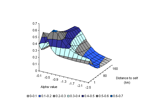
Chart B1 and Chart B2 present the sensitivity of the estimate of the proportion of the productivity gap between Australia and the United States explained by the proximity indicator to changes in the two parameters, ![]() and
and ![]() . These suggest that the estimate is generally robust within the range of two standard errors of the parameter estimates in Table B1.
. These suggest that the estimate is generally robust within the range of two standard errors of the parameter estimates in Table B1.
Chart B1: Proportion of the productivity gap explained by the
proximity indicator Contour Map
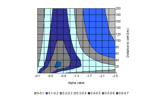
Chart B2: Proportion of the productivity gap explained by the
proximity indicator 3D Surface
1 For instance, in 2000, around 27 per cent of Australian workers were part time, compared with around 13 per cent for the US workforce.
2 The scaling of the data has a negligible impact on the key marginal effects presented later in this paper.
3 The Conference Board and Groningen Growth and Development Centre, Total Economy Database, January 2006, http://www.ggdc.net.
4 US data are restricted to the number of people over 25 years holding a bachelor’s degree or better.
5 This was done using an inverse tan transformation
of the likelihood parameter ![]() :
:
![]()
This smoothly constrained ![]() to values between 0 and 2 and, consequently, limited the likelihood procedure to finding any maximum that might exist in that range.
to values between 0 and 2 and, consequently, limited the likelihood procedure to finding any maximum that might exist in that range.